(This is part 4 of the “Stages of the Anthropocene, Revisited” Series (SotA-R).)
The purpose of this series is an update of the mid- and long-term prediction of aspects of the global climate relevant for the prospects of continuing human civilization in Stages of the Anthropocene. The idea is to develop a model that can be relatively easily expanded, fine-tuned, and corrected when new or better information becomes available. The present episode in the series consists of a number of notes of a relatively technical nature on how to build this model.
CO₂ emissions and economic growth
The level of CO₂ emissions in a country depends primarily on wealth. There is no significant relation between changes on the short term, however. The correlation between yearly CO₂ (equivalent) growth and economic growth between 1980 and 2016 for the 164 countries in my data set is as low 0.058.1 What explains this low correlation is probably that at such short time scales there are too many other factors influencing CO₂ emissions and that emissions don’t always immediately respond to economic changes.
That economic growth almost completely determines CO₂ emissions in the long run becomes clear if one looks at the correlation between wealth (measured as GDP) and emissions on the other hand. That correlation (for the same 164 countries in all years from 1980 to 2016) is 0.94. The relation appears almost linear and simply multiplying GDP with 3×10⁻¹⁰ results in a pretty good estimate of CO₂ emissions. There are important deviations, however, as well as local circumstances that must be taken into account, and therefore, the best approach to simulate CO₂ emissions of some country in some year 1 is to take the ratio of the predicted emissions in that country for years 1 and 0 and multiply that ratio with the given or modeled emissions in year 0. In practice, this is the same as taking the (year-to-year) economic growth rate and using that as the emission growth rate as well.2
emission reduction
Thus far, efforts to reduce CO₂ emissions have been mostly inconsequential, but presumably this will slowly change in the coming decade(s). Hence, CO₂ emissions should be modeled as a function of economic growth and reduction efforts. The latter themselves depend – among others – on economic growth and the level of wealth, however, as in times of economic crisis (or worse) investment in clean technology tends to dry up and because poorer countries are less able to make such investments even in the best circumstances.
When it comes to emission reduction, it may be necessary to consider multiple scenarios. A reasonable, medium effort scenario can double as the yardstick for the others. In that medium effort scenario every time some “thing” reaches the average replacement age for that kind of thing, it is replaced by a zero-emission alternative or whatever is the best available alternative (and the bulk of new “things” that are not replacements are as carbon-neutral as possible as well). It is important to realize that any replacement schedule faster than that would mean discarding things before their normal economic life span, and therefore, before it would have reached its expected return on investment. In other words, replacing “things” faster than this medium effort scenario means “throwing away” money and would thus require substantial government subsidies. (Of course, it would be much better in the long run to “throw away money” in this sense and to make a very big effort to reduce emissions as quickly as possible, but unfortunately, in business and politics no one is genuinely interested in the long run.)
There are significant differences in the average replacement age of different kinds of “things”. Cars tend to be replaced every 8 years (on average!), but electric power plants have an expected economic life span of 40 years or even more. Hence, to find the yearly average medium effort emission reduction – that is, the expected yearly CO₂ reduction in the medium effort scenario – data is needed on CO₂ emissions per sector and on the average replacement age of the main emitting devices used in that sector. All of this data can be found on the internet,3 but there is another problem: some emissions cannot really be reduced significantly (or at all) at the current state of technology. There are no good alternatives for coal in steel production, for example, and cement making and agriculture emit enormous amounts of CO₂ as well. In total, it appears that at least 36% of current global emissions belong to this kind. Even with our best effort, we cannot reduce those, because we don’t have the technology necessary, nor replacements for the processes and/or products involved.
Taking average replacement schedules and expected economic life spans into account, the remainder can be reduced by approximately 3.5% of the current level per year, but that percentage drops when it approaches the bottom level. That bottom level won’t be 36% in the long run, however, as it should be expected that on decadal time scales some relevant technologies will be developed and become viable, and that solar- (or nuclear-) powered carbon capture might reduce net emissions by a few percent as well. The further into the future, the lower that bottom level might be.
As mentioned, in addition to this medium effort scenario, it is probably a good idea to consider some further scenarios. A high effort scenario is roughly the maximum yearly CO₂ reduction that is economically feasible (but also involves more investment in the development of relevant new technologies). My calculations suggest that this is just below 5% in the first year (and then very slowly dropping as in the medium effort scenario). A low effort scenario doesn’t have an obvious target value, but 75% of the medium effort seems reasonable. Anything below that is more appropriately called a “no effort” scenario. (At present, we’re nowhere near the low effort scenario, by the way. In the contrary, we’re still investing in more fossil fuel burning infrastructure.)
The following graph shows yearly global CO₂ reductions in these three scenarios (current emissions indexed at 100) for the next century if everything else remains equal (which is an absurd assumption in this context, of course, but remember that the present goal is just one small piece of the puzzle).
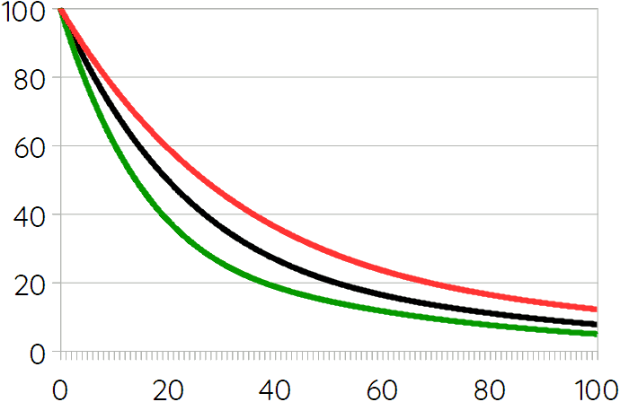 The medium effort scenario (black line) would put an additional 950 gigatonnes CO₂-equivalent in the atmosphere by 2050. The high effort scenario 810, and the low effort scenario 1050. This would lead to between 2.5 and 3°C of average global warming. But note that the “everything else stays equal” condition also implies that there is no economic growth whatsoever, which is impossible under capitalism (except during a crisis).
These are still further scenarios that need to be taken into account, however. For example, a superlow effort scenario starting at 1% yearly reduction would lead to 1300 gigatonnes CO₂-equivalent by 2050. However, it is nearly impossible in practice to use all of these scenarios in the final model of carbon emissions in stage 1 of the anthropocene.
It seems plausible to me, that the effort made by some country depends on public opinion and financial/economic realities. Climate change-related disasters are expected to change public opinion to demand greater effort, while economic crisis and/or widespread civil unrest will make a country gravitate towards a no effort scenario. This would probably be a good starting point for the overall model because it is relatively easy to implement, and it would also be relatively easy to make various small changes to test it for robustness. Because I doubt that the economic reality will ever be such that the high effort scenario becomes a realistic possibility, it seems to me that CO₂ reductions can be modeled as being in between 0 (no effort) and the value given by the medium effort scenario, where low or negative economic growth pulls towards 0 and time pulls towards medium effort (because with time the effects of climate change will become more apparent).
modeling economic growth
From the preceding two sections it follows that economic growth is the key variable in the model. Recall that the linear correlation between wealth and CO₂ emissions is as high as 0.98 and that economic growth largely determines how much a country can spend on replacing things (machines, infrastructure, and so forth) by carbon-neutral alternatives. Hence, to predict CO₂ emissions in stage 1 of the anthropocene – or even just until 2050, we need a model of economic growth. That, unfortunately, is not so easy, but a relatively simple model consisting of a merely four components may go a long way. Those four components are: (1) a base rate of economic growth for a given country, which starts at its growth rate for the past decade or so and gradually tends towards the global average; (2) an estimate of the likelihood of economic crisis and/or stagnation; (3) an estimate of the expected economic effects of climate-change-related disasters; and (4) an estimate of the likelihood of widespread unrest, civil war, or – in extreme cases – societal collapse. The first of these would – as the term “base rate” already suggests – be the normal scenario, while (2) to (4) would represent possible major deviations therefrom.
The best indicator of the likelihood of economic crisis or stagnation (i.e. 2) is the private debt to GDP ratio. As Richard Vague has shown, crisis follows when private debt is roughly 150% of GDP or more,4 and even if crisis is somehow (usually temporarily) avoided, further economic growth becomes virtually impossible and the country becomes what Steve Keen calls a “debt zombie”.5 Insufficiently drastic restructuring in and after an economic crisis will also change a country into a debt zombie. Furthermore, even without a crisis, high levels of private debt slowly strangle an economy, depressing economic growth.6 Because the effects of crisis and stagnation more or less average out on the longer run, it might actually not be necessary to model the probability of various crisis scenarios, which would significantly complicate the overall model. Instead, it might be sufficient to add an equation that depresses economic growth in case of high levels of private debt, such that when the latter exceeds 150% of GDP economic growth reaches 0.7 This, of course, means that I need to have a model of the development of private debt. I have some ideas about how to make that model, but this needs further work.
The third of the three components mentioned above is an estimate of expected economic effects of climate-change-related disasters. This is, of course, where the previous two episodes in this series come in the picture. Drought, extreme heat, tropical cyclones, extreme weather, an so forth can all have an impact on a country’s economy. How large that impact is depends on the kind of disasters and the proportion of the country’s territory and population they are expected to affect. The Philippines, Taiwan, and much of the Caribbean are expected to experience much cyclone-related damage, possibly crippling their economies within a few decades. Indonesia and Venezuela (among others) will likely be too hot for any kind of manual labor half the year. And huge swaths of land will be too dry to feed their current populations in two decades from now. How exactly all of this affects the economies involved is a difficult question. Perhaps, the best approach is to make the model in such a way that it is easy to try out the effects of different assumptions on the economic effects of (different kinds of) disaster.
The fourth component concerns the likelihood of civic unrest and so forth. This may actually very well be the most important aspect of the model, because civil war (as an extreme case of civic unrest) leads to greater CO₂ emission reductions than any non-violent scenario could ever establish. Looking at the economic effects of civil wars in the past decades, it becomes clear that on average, civil war decreases a country’s GDP with some 15% per year, but that this can easily surpass 50% or even 60% in extreme cases (such as Libya in 2011, for example). Even lower intensity violent conflict tends to cause economic damage in the range of 5% per year. However, in the long run there appears to be a limit – countries aren’t destroyed completely and the high intensity violence leading to an average of 15% economic destruction per year rarely lasts for more than 4 years. Typically, a civil war wipes away roughly half of a country’s economy. This, obviously, has big effects on CO₂ emissions as those are largely determined by the state of the economy, and consequently, what is needed is a model of the likelihood of civil war and other kinds of high-intensity violent civic unrest. Contrary to economic crisis and stagnation, the effects of civil war hardly average out, and consequently it might be necessary to develop different scenarios for different civil wars with different probabilities and different emission outcomes (but see below).
civic unrest
So, what determines the likelihood of civil war and other kinds of violent civic unrest? As in case of economic growth, it is probably best to distinguish some kind of base rate from the factors that might cause deviations therefrom such as food scarcity, economic crises, spill-over from conflicts in neighboring countries, and so forth. That base rate, then, is the likelihood of widespread violent civic unrest in a country if none of those deviation-causing factors play a role.
Probably the best indicator of violent civic unrest in a country is that it has already experienced civil war or similar kinds of conflict in the recent past. The more recent that conflict is, the more likely it is that it will flare up again. This kind of data is made available by the Uppsala Conflict Data Program, among others. I don’t believe that this is sufficient, however. All of the countries that experienced civil wars in the past decades rank extremely low on the Democracy Index made by the Economist Intelligence Unit. Furthermore, countries that experienced significant unrest of lesser intensity also tend to score relatively low. Hence, a low ranking on the Democracy Index might be a good secondary indicator. Other factors that may influence the likelihood of violent conflict include the prevalence of violence in a country (measured, for example, by its murder rate), the frequency of incidents of domestic terrorism, the availability of weapons (especially privately-owned weapons), and perhaps certain cultural factors, although I’m not sure which ones.
The “deviation-causing factors” mentioned above are already part of the model. Food scarcity is mainly caused by drought (but also by food price speculation), which was also mentioned as a possible depressor of economic growth. Economic crisis was a key issue in the previous section. And spill-over from adjacent conflicts is just an interaction effect added to the civic unrest sub-model. Perhaps, there are other major factors that could cause violent civic unrest that need to be taken into account (and that aren’t incorporated in the base rate already), but right now I have no idea what those could be.
too many scenarios
The biggest problem for the model is dealing with all the probabilities. To illustrate the problem, consider the following example. Let’s say there are two countries in the model. The temporal resolution is single years and the time period modeled is thirty years. There is one probabilistic, dichotomous variable – that is, there is one kind of event that either occurs or doesn’t in any given year with probability P for occurrence and 1–P for non-occurence. In that case the number of possible model outcomes is the total number of different combinations of occurrences of that event, which is 2 to the power of 2×30. The first “2” represents the occurrence/non-occurrence dichotomy (i.e. two states); the second “2” the number of countries; and the “30” the number of model steps (i.e. years). 2 to the power of 60 is a bit over one quintillion. That’s a stupendously big number, and that’s with just two countries and one probabilistic, dichotomous variable.
I don’t have the computing power, nor the software or the skills necessary to model all relevant probabilities, so I’ll need to make some shortcuts. As mentioned, the probability of economic crisis can probably be replaced by a non-probabilistic module that translates private debt into less economic growth. The probability of violent conflict cannot be dealt with in a similar way, however. Either violent civic unrest occurs or it doesn’t and if it occurs then this changes things, possibly even drastically. Actually, this isn’t exactly right, because violent conflict can have various levels of intensity. Because low-intensity conflict has only relatively minor effects and tends to consists of many minor incidents that sort of average out on the long run, that kind of civic unrest can be modeled non-probabilistically as a minor influence on economic growth. The issue is high-intensity conflict, such as civil war or societal conflict, however – that’s the kind of conflict that destroys half a country’s economy (or even more) and causes waves of refugees. And the probabilistic nature thereof cannot be eliminated.
The most obvious work-around is to drastically reduce the spatial and temporal resolution, but that would create other difficulties, and it is quite doubtful whether the resolution can be reduced enough without making the model useless. A temporal resolution of 5 years would be rough, but might still be acceptable, and countries could probably be grouped into between 15 and 20 regions. At that kind of scale, civic unrest cannot be treated as a dichotomous variable, however, but it becomes necessary to distinguish probabilities of low, medium, and high-violence scenarios. This results in 3 to the power of 6 times the number of regions (i.e. between 15 and 20), which is a number with between 42 and 57 digits, so that’s obviously not an option. What may be possible in case of such a model, on the other hand, is to develop a limited number of scenarios that represent a random selection of those ludicrously many possible scenarios. This would at least give an indication of what kind of uncertainty margins there are.
But before going there, it may be best to develop a non-probabilistic version of the model first by multiplying risks with their effects. This would be relatively easy to do and would probably get us close to the peak in the curve (i.e. average expected CO₂ emissions by 2050, assuming that expectations according to the model are normally distributed). If that model is made in such a way that it is easy to systematically and/or specifically manipulate risks it would also be possible to test for one particular kind of robustness. If it would happen to turn out that quite extreme scenarios don’t deviate extremely from the average expectation (i.e. the peak in the curve) then all the aforementioned difficulties are really quite irrelevant.
Anyway, if you have read all of the above, you’ll probably realize that it’s going to take a while to collect the data, build and calibrate the model, and produce some results (even if I would be able to work on it full time). So the next episode in this series won’t probably be published any time soon.
If you found this article and/or other articles in this blog useful or valuable, please consider making a small financial contribution to support this blog, 𝐹=𝑚𝑎, and its author. You can find 𝐹=𝑚𝑎’s Patreon page here.
Notes
- Data source: Our World in Data.
- This section was corrected on September 29. The original correlations and calculation (i.e. formula) given here were based on an error in the data.
- For emissions per sector, see Our World in Data, for example.
- Richard Vague (2019). A Brief History of Doom: Two Hundred Years of Financial Crises (Philadelphia: University of Pennsylvania Press).
- Steve Keen (2017). Can We Avoid Another Financial Crisis? (Cambridge: Polity).
- See Rent, Debts, and Power.
- Crisis followed by minor recovery and stagnation due to insufficient debt restructuring would average out to the same. Only when private debt is significantly decreased becomes economic growth possible again.